Computing on the Dynex Neuromorphic Platform: Image Classification

12 min readSep 14, 2023

Computing on Quantum or neuromorphic systems is fundamentally different than using traditional hardware and is a very active area of research with new algorithms surfacing almost on a weekly basis. In this article we will use the Dynex SDK (beta) to perform an image classification task using a transfer learning approach based on a Quantum-Restricted-Boltzmann-Machine (“QRBM”) based on the paper “A hybrid quantum-classical approach for inference on restricted Boltzmann machines”. It is a step-by-step guide on how to utilize neuromorphic computing with Python using PyTorch. This example is just one of multiple possibilities to perform machine learning tasks. However, it can be easily adopted to other use cases.

Requirements

To compute on the Dynex Platform, the Dynex SDK (beta) is required. It can be installed with:

pip install dynex

You will also need to configure your API as explained in the Dynex SDK Wiki.

Environment: PyTorch

We will be using a Jupyter Notebook to perform all computations. The Dynex SDK (beta) comes with a PyTorch layer class which can be seamlessly used in PyTorch models. We therefore also need PyTorch installed on our Python environment.

Imports

We will import the libraries which will be used throughout this example:

import math
import os
import numpy as np
import matplotlib.pyplot as plt

# PyTorch:
import torch
import torch.nn as nn
from torchvision.transforms import ToTensor
from torch.utils.data import random_split
from torch.utils.data import DataLoader
from torch.nn import Module
from torchvision import transforms

# Sklearn:
from sklearn.metrics import classification_report
from sklearn.linear_model import LogisticRegression

# Dynex:
from HybridQRBM.pytorchdnx import dnx
from HybridQRBM.optimizers import RBMOptimizer
from HybridQRBM.samplers import DynexSampler

Dataset

We will use the MNIST database, which is a large database of handwritten digits that is commonly used for training various image processing systems. It is also widely used for training and testing in the field of machine learning and therefore constitutes a good benchmark test-set. PyTorch offers this dataset per default. We also apply a simple data_transformer to convert the images from gray-scale to black and white:

from torchvision.datasets import MNIST

# data transformer:
class ThresholdTransform(object):
  def __init__(self, thr_255):
    self.thr = thr_255 / 255.  

  def __call__(self, x):
    return (x > self.thr).to(x.dtype)  

data_transformer = transforms.Compose([
        transforms.ToTensor(),
        ThresholdTransform(thr_255=128) 
    ])

# download the data:
trainData = MNIST(root="data", train=True, download=True, transform=data_transformer)
testData = MNIST(root="data", train=False, download=True, transform=data_transformer) 

print("[INFO] MNIST dataset lodaed")

>> [INFO] MNIST dataset lodaed

Model Definition

Boltzmann machine is a powerful machine learning model with many real-world applications, for example by constructing deep belief networks. We will use an adopted version, a Quantum-Restricted-Boltzmann-Machine for our example as published in “A hybrid quantum-classical approach for inference on restricted Boltzmann machines”. It is capable of learning a probability distribution that represents the input data and therefore can be used for dimensionality reduction, or to reconstruct images. Albeit it would be possible to stack the labels onto the visual layer of the network, we will demonstrate a transfer learning approach. We will build a classification pipeline with a QRBM as feature extractor by using the hidden nodes as inputs for a Logistic Regression classifier.

The QRBM utilizes the Dynex Neuromorphic Platform for energy optimized initialization of the Gibbs sampling steps rather than random initialization. As a result, we will demonstrate that only 1 training epoch is already sufficient to achieve a model accuracy of 95%+.

Parameters

We therefore define the training parameters as followed:

INIT_LR    = 1e-3    # initial loss rate of the optimizer
BATCH_SIZE = 10000   # number of images per batch
EPOCHS     = 1       # number of training epochs
device = "cpu"       # no GPU needed, we compute on the Dynex Platform

The Dynex PyTorch layer also comes with optimizer and sampler classes. We define them with:

optimizer = RBMOptimizer(
                learning_rate=0.05,
                momentum=0.9,
                decay_factor=1.00005,
                regularizers=()
            );

sampler = DynexSampler(mainnet=True, 
               num_reads=100000, 
               annealing_time=200,  
               debugging=False, 
               logging=True, 
               num_gibbs_updates=1, 
               minimum_stepsize=0.002);

The sampler class also defines the settings which are being used for the computations on the Dynex platform. We want to utilize 100,000 Dynex chips for a period of 200 integration steps and a minimum step-size of 0.002 for each forward Euler ODE integration step. More background and information can be found in sampling options and below in further reading.

We can now define the model. It consists of just one Dynex neuromorphic layer which is designed to find energy ground states for the entire batch of images — all of which are computed in parallel on the Dynex Platform. Technically, it is a QRBM (Quantum Restricted Boltzmann Machine) Layer returning the weights of the hidden layer. This layer is capable to reconstruct images. To classify those, we will apply a simple logistic regression model based on the hidden layers of the QRBM in a second step.

class QModel(nn.Module):
    def __init__(self, n_hidden, steps_per_epoch, sampler, optimizer):
        super().__init__();
        # Dynex Neuromporphic layer
        self.dnxlayer = dnx(n_hidden, steps_per_epoch, sampler=sampler, optimizer=optimizer); 
        
    def forward(self, x):
        x = self.dnxlayer(x);
        return x

Step 1: Model Training — QRBM

To train our model, we define the train and test loaders first:

# initialize the train and test data loaders
trainDataLoader = DataLoader(trainData, shuffle=True, batch_size=BATCH_SIZE)
testDataLoader = DataLoader(testData, batch_size=BATCH_SIZE)

These will load 10,000 images in 6 batches (steps_per_epoch) for our training. Due to the parallel nature of the Dynex platform, data from all batches are combined and then all 60,000 images sampled at once in parallel. We choose 300 hidden nodes for our model:

steps_per_epoch = len(trainDataLoader.dataset) // BATCH_SIZE
model = QModel(300, steps_per_epoch, sampler, optimizer);

Technically, more epochs will lead to increased accuracy, that’s why we construct a training loop. In our example we will demonstrate that just one training epoch is sufficient to achieve a high level of accuracy. The training loop is similar to any other PyTorch based training:

for e in range(1, EPOCHS+1):
    print('EPOCH',e,'of',EPOCHS);
    # set the model in training mode
    model.train()
    # loop over the training set
    for (x, y) in trainDataLoader:
        # send the input to the device
        (x, y) = (x.to(device), y.to(device))
        # perform a forward pass and calculate the training loss
        pred = model(x);
    
print('FOUND MODEL ACCURACY:',np.array(model.dnxlayer.acc).max(),'%')

This is where the magic happens:

EPOCH 1 of 1
DynexQRBM PyTorch Layer | batch data appended: 1
DynexQRBM PyTorch Layer | batch data appended: 2
DynexQRBM PyTorch Layer | batch data appended: 3
DynexQRBM PyTorch Layer | batch data appended: 4
DynexQRBM PyTorch Layer | batch data appended: 5
DynexQRBM PyTorch Layer | batch data appended: 6
DynexQRBM PyTorch Layer | end of batch, sampling... 60000 x 784
[DYNEX] MODEL CONVERTED TO QUBO
[DYNEX] PRECISION SET TO 1e-07
[DYNEX] QUBO: Constant offset of the binary quadratic model: 0.0
[DYNEX] SAMPLER INITIALISED
[DYNEX] MALLOB: JOB CREATED:  3927
[ÐYNEX] SUBMITTING JOB - UPLOADING JOB FILE...

The DynexQRBM PyTorch Layer collects all 6 batches and initiates the sampling of 60,000 training samples. Technically a computation file is being generated and submitted by the Dynex SDK (beta) to the Dynex platform. This sampling file can also be found locally on your machine in folder /tmp:

During the sampling, the progress can be monitored, because we defined the model with the parameter “logging=True”. The workers performing computations, the current energy ground state, number of used chips and more are being displayed. This output can also be silenced by setting “logging=False”:

╭────────────┬───────────┬───────────┬─────────┬────────┬─────────┬───────┬───────┬───────────┬──────────────╮
│   DYNEXJOB │   ELAPSED │   WORKERS │   CHIPS │      ✔ │   STEPS │   LOC │     ✔ │    ENERGY │            ✔ │
├────────────┼───────────┼───────────┼─────────┼────────┼─────────┼───────┼───────┼───────────┼──────────────┤
│       3927 │      0.80 │        14 │  351456 │ 101408 │     200 │ 49296 │ 49480 │ 888846747 │ 883276358.00 │
╰────────────┴───────────┴───────────┴─────────┴────────┴─────────┴───────┴───────┴───────────┴──────────────╯
╭───────────┬───────────────┬─────────┬────────┬──────────────┬───────────┬───────────────┬──────────╮
│    WORKER │       VERSION │   CHIPS │    LOC │       ENERGY │   RUNTIME │   LAST UPDATE │   STATUS │
├───────────┼───────────────┼─────────┼────────┼──────────────┼───────────┼───────────────┼──────────┤
│ 130400088 │ 2.3.0.OZM.124 │   16128 │  49480 │ 888846747.00 │  0.05 min │    29.00s ago │  STOPPED │
├───────────┼───────────────┼─────────┼────────┼──────────────┼───────────┼───────────────┼──────────┤
│ 130400072 │ 2.3.0.OZM.124 │    8064 │  50781 │ 889705545.00 │  0.05 min │    33.00s ago │  STOPPED │
├───────────┼───────────────┼─────────┼────────┼──────────────┼───────────┼───────────────┼──────────┤
│ 130400118 │ 2.3.0.OZM.124 │    4640 │  50427 │ 892108390.00 │  0.07 min │    19.00s ago │  STOPPED │
├───────────┼───────────────┼─────────┼────────┼──────────────┼───────────┼───────────────┼──────────┤
│ 130400196 │ 2.3.0.OZM.123 │    8064 │ 114556 │ 892542824.00 │  0.07 min │     0.00s ago │  STOPPED │
├───────────┼───────────────┼─────────┼────────┼──────────────┼───────────┼───────────────┼──────────┤
│ 130400059 │ 2.3.0.OZM.124 │    5952 │  50995 │ 893735038.00 │  0.07 min │    36.00s ago │  STOPPED │
├───────────┼───────────────┼─────────┼────────┼──────────────┼───────────┼───────────────┼──────────┤
│ 130400085 │ 2.3.0.OZM.123 │    8064 │ 114777 │ 894401041.00 │  0.07 min │    29.00s ago │  STOPPED │
├───────────┼───────────────┼─────────┼────────┼──────────────┼───────────┼───────────────┼──────────┤
│ 130400100 │ 2.3.0.OZM.122 │    9056 │ 114605 │ 894505283.00 │  0.05 min │    27.00s ago │  STOPPED │
├───────────┼───────────────┼─────────┼────────┼──────────────┼───────────┼───────────────┼──────────┤
│ 130400016 │ 2.3.0.OZM.124 │   16256 │  50518 │ 895750003.00 │  0.05 min │    45.00s ago │  STOPPED │
├───────────┼───────────────┼─────────┼────────┼──────────────┼───────────┼───────────────┼──────────┤
│ 130400136 │ 2.3.0.OZM.124 │    7296 │  50353 │ 895906853.00 │  0.07 min │    13.00s ago │  STOPPED │
├───────────┼───────────────┼─────────┼────────┼──────────────┼───────────┼───────────────┼──────────┤
│ 130400113 │ 2.3.0.OZM.123 │    4640 │ 114682 │ 896683705.00 │  0.07 min │    21.00s ago │  STOPPED │
├───────────┼───────────────┼─────────┼────────┼──────────────┼───────────┼───────────────┼──────────┤
│ 130400124 │ 2.3.0.OZM.123 │    9408 │ 114796 │ 897065634.00 │  0.05 min │    18.00s ago │  STOPPED │
├───────────┼───────────────┼─────────┼────────┼──────────────┼───────────┼───────────────┼──────────┤
│ 130400102 │ 2.3.0.OZM.124 │     576 │  52086 │ 897810330.00 │  0.13 min │    21.00s ago │  STOPPED │
├───────────┼───────────────┼─────────┼────────┼──────────────┼───────────┼───────────────┼──────────┤
│ 130399889 │ 2.3.0.OZM.124 │   13568 │  51925 │ 898257597.00 │  0.83 min │    30.00s ago │  STOPPED │
├───────────┼───────────────┼─────────┼────────┼──────────────┼───────────┼───────────────┼──────────┤
│ 130400080 │ 2.3.0.OZM.123 │     320 │ 115261 │ 898325767.00 │  0.07 min │    30.00s ago │  STOPPED │
├───────────┼───────────────┼─────────┼────────┼──────────────┼───────────┼───────────────┼──────────┤
│ 130400108 │ 2.3.0.OZM.123 │   10752 │ 114954 │ 898424784.00 │  0.10 min │    20.00s ago │  STOPPED │
├───────────┼───────────────┼─────────┼────────┼──────────────┼───────────┼───────────────┼──────────┤
...

Once completed, the sampling results are being collected and applied to the model:

[DYNEX] FINISHED READ AFTER 0.80 SECONDS
[DYNEX] MALLOB: JOB UPDATED: 3927 STATUS: 2
[DYNEX] WAITING 30 SECONDS FOR ALL WORKERS TO SUBMIT READS...
[DYNEX] READING  40 VOLTAGES...
[DYNEX] SAMPLESET LOADED
DynexQRBM PyTorch Layer | applying sampling result... 60000 x 784
DynexQRBM PyTorch Layer | SME: 0.009717 ACCURACY: 99.028318%
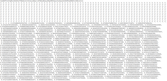
FOUND MODEL ACCURACY: 99.0283181717132 %

The layer is automatically using the voltage assignments with the lowest energy ground state for setting the initial conditions of the Gibs sampling step. As we can observe from above, the lowest energy confirmed was 883,276,358.00. If we are interested, we can inspect the voltages of this assignment by opening the according file in /tmp:

Which, when opened, shows us the sampling result with values for the initial assignments:

It also shows us which worker (miner wallet address) has contributed this assignment. The Dynex PyTorch layer generates a logfile documenting the progress, which is located in /log:

2023-09-14 14:06:04,307:INFO:DynexQRBM PyTorch Layer | batch data appended:  1
2023-09-14 14:06:05,329:INFO:DynexQRBM PyTorch Layer | batch data appended:  2
2023-09-14 14:06:06,385:INFO:DynexQRBM PyTorch Layer | batch data appended:  3
2023-09-14 14:06:07,578:INFO:DynexQRBM PyTorch Layer | batch data appended:  4
2023-09-14 14:06:08,597:INFO:DynexQRBM PyTorch Layer | batch data appended:  5
2023-09-14 14:06:09,897:INFO:DynexQRBM PyTorch Layer | batch data appended:  6
2023-09-14 14:09:21,981:INFO:Dynex Platform: sampled response: energy = -3.0913626279046515
2023-09-14 14:11:29,249:INFO:DynexQRBM PyTorch Layer | SME:  0.009716818282868035
2023-09-14 14:11:29,250:INFO:DynexQRBM PyTorch Layer | ACCURACY: 99.0283181717132%

Each computing job is identified by its job number, in our example 3927 (see above). Details of the computation are also accessible in real-time through the Dynex website or selected pool operator pages:

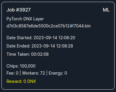
As we can see, was the computation finished after 00:02:08.

Visualizing Training Progress

Our example requires just one training epoch, however we can visualize the evolution of the Mean Squared Error rate (MSE) with this code:

plt.figure()
plt.plot(model.dnxlayer.errors, label='dnxModel')
plt.xlabel('epoch')
plt.ylabel('MSE')
plt.legend()
plt.show()
print(model.dnxlayer.errors)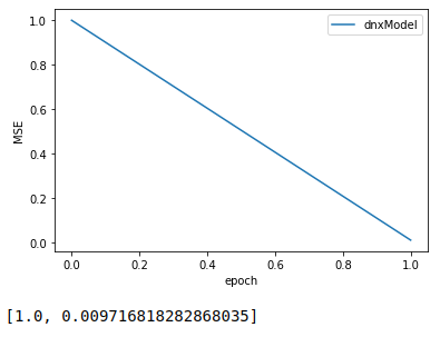

Step 2: Building the classifier

Visualizing the test data set

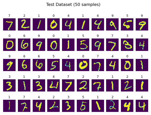
The test set consists of 10,000 test samples, which are not included in the training data set. We can inspect the test set with the following code:

num_samp = 0;
num_batches = 0;
for batch_idx, (inputs, targets) in enumerate(trainDataLoader):
    num_samp += len(inputs);
    num_batches += 1;
    
print(num_batches,' batches total', num_samp,'images in total, one batch',len(inputs),'images')

# last batch:
fig = plt.figure(figsize=(10, 7));
fig.suptitle('Test Dataset (50 samples)', fontsize=16)
rows = 5;
columns = 10;

for j in range(0,50):
    fig.add_subplot(rows, columns, j+1)
    plt.imshow(inputs[j][0])
    marker=str(targets[j].tolist())
    plt.title(marker)
    plt.axis('off');
    
plt.show();

>>> 1  batches total 10000 images in total, one batch 10000 images

Which generates the following output (first 50 samples, label on top):

Transfer Learning: QRBM Hidden Layers to Logistic Regression

As discussed above, will we build a classification pipeline with a QRBM as feature extractor by using the hidden nodes as inputs for a Logistic Regression classifier. As a first step will we convert test set samples into the Logistic Regression data format:

data = [];
data_labels = [];
error = 0;
for i in range(0, 150):
    inp = np.array(inputs[i].flatten().tolist()); 
    tar = np.array(targets[i].tolist())
    data.append(inp)
    data_labels.append(tar)
data = np.array(data)
data_labels = np.array(data_labels)

Then we extract the hidden layers from our QRBM

# extract hidden layers from RBM:
hidden, prob_hidden = model.dnxlayer.sampler.infer(data)

And train a simple logistic regression classifier:

# Logistic Regression classifier on hidden nodes:
t = hidden * prob_hidden
clf = LogisticRegression(max_iter=10000)
clf.fit(t, data_labels)
predictions = clf.predict(t)
print('Accuracy:', (sum(predictions == data_labels) / data_labels.shape[0]) * 100,'%')

>>> Accuracy: 99.33333333333333 %

The final classifier yields an accuracy of 99.33% on our test data-set samples. Inspecting predictions vs. target values:

# inspect predictions:
print('target   :',data_labels[:30])
print('predicted:',predictions[:30])

>> target   : [7 2 1 0 4 1 4 9 5 9 0 6 9 0 1 5 9 7 3 4 9 6 6 5 4 0 7 4 0 1]
>> predicted: [7 2 1 0 4 1 4 9 4 9 0 6 9 0 1 5 9 7 8 4 9 6 6 5 4 0 7 4 0 1]

To validate the quality of the underlying QRBM, we can use the trained model to reconstruct our images from the test data-set:

# reconstruct / predict our samples:
_, features = model.dnxlayer.sampler.predict(data, num_particles=10,num_gibbs_updates=1)

Which can then be visualized:

fig = plt.figure(figsize=(10, 7));
fig.suptitle('Reconstructed Dataset (50 samples)', fontsize=16)
rows = 5;
columns = 10;
for i in range(0,50):
    fig.add_subplot(rows, columns, i+1)
    plt.imshow(features[i].reshape(28,28))
    marker=str(predictions[i])+' (t='+str(data_labels[i])+')'
    plt.title(marker)
    plt.axis('off');
plt.show()

It outputs the QRBM’s reconstructed images:

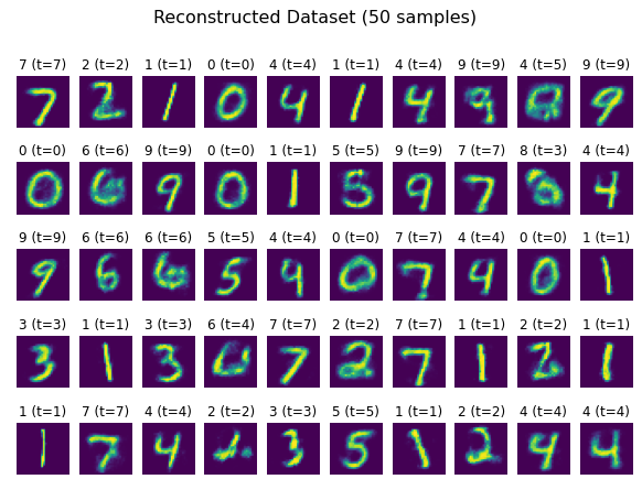
Reconstructed images. Label: Predicted (expected)

The visual inspection of our reconstructed images validates the quality of the QRBM. The Dynex Pytorch layer also allows saving and loading of models. Especially for larger models which have been trained for a longer period of time, models can be saved and later loaded for predictions.

Saving a Model

Our model can be saved with the following, default PyTorch based command:

torch.save(model, './checkpoint/ckpt.pth')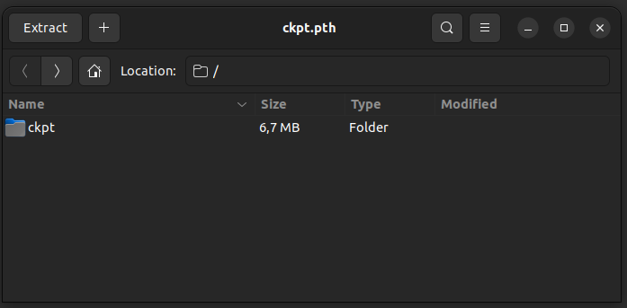

This can be done during the training process, or after all epochs have been trained.

Loading and Using a Model

At any later point, we can simply load a pre-trained model and perform predictions or additional training steps:

testmodel = torch.load('./checkpoint/ckpt.pth');

We can verify that the loaded model ‘testmodel’ equals our model above:

# verify that model was correctly loaded:
testmodel.dnxlayer.weights == model.dnxlayer.weights

>> array([[ True,  True,  True, ...,  True,  True,  True],
       [ True,  True,  True, ...,  True,  True,  True],
       [ True,  True,  True, ...,  True,  True,  True],
       ...,
       [ True,  True,  True, ...,  True,  True,  True],
       [ True,  True,  True, ...,  True,  True,  True],
       [ True,  True,  True, ...,  True,  True,  True]])

The loaded model can also be used for image reconstruction (predicting features with the QRBM) or for classification in the same fashion:

_, features = testmodel.dnxlayer.sampler.predict(data, num_particles=10,num_gibbs_updates=1)
# extract hidden layers from RBM:
hidden, prob_hidden = testmodel.dnxlayer.sampler.infer(data)
# Logistic Regression classifier on hidden nodes:
from sklearn.linear_model import LogisticRegression
t = hidden * prob_hidden
clf = LogisticRegression(max_iter=10000)
clf.fit(t, data_labels)
predictions = clf.predict(t)
print('Accuracy:', (sum(predictions == data_labels) / data_labels.shape[0]) * 100,'%')

>> Accuracy: 99.33333333333333 %

Similar for reconstruction:

fig = plt.figure(figsize=(10, 7));
fig.suptitle('Reconstructed Dataset (50 samples)', fontsize=16)
rows = 5;
columns = 10;
for i in range(0,50):
    fig.add_subplot(rows, columns, i+1)
    plt.imshow(features[i].reshape(28,28))
    marker=str(predictions[i])+' (t='+str(data_labels[i])+')'
    plt.title(marker)
    plt.axis('off');
plt.show()

Which outputs:

Reconstructed images with the loaded model. Label: Predicted (expected)

We hoped you enjoyed reading this article. All codes are also available on our GitHub repository. If you want to learn more, visit the Dynex SDK Wiki. You can also get in touch with us on one of our channels.